It goes without saying that cables are a critical part of any electrical system. Their simplicity and lack of “fancy” parts can mislead you into thinking they're one of the simpler components to design. However, one of the greatest challenges and thus a major source of innovation in the early days of the power grid was in cable design. Every power grid in the world is built around that cable design problem. We will ultimately discuss what this innovation is, after it has been put into context.
Part 1: How Cables Fail (Electrically)
Let's start with how cables fail. A cable's sole purpose is to transmit power from the source to the load. But to understand failure, we need to look past power itself and break it down into its two fundamental components: current and voltage. P = VI, where P is power, V is voltage, and I is current.Therefore, a cable transmits power by maintaining a voltage across its length and conducting a current through its lines. This means there are two primary electrical failure modes (we'll leave mechanical ones for later): a cable can fail because of a voltage it can't withstand, or a current it can't carry.
1. Voltage Failure
The voltage rating of a cable is determined by the insulation material between the conductors. If the voltage across the cable is too high, it can overwhelm the insulation, leading to a catastrophic breakdown, such as an arc or short circuit.
2. Current Failure
The current rating, on the other hand, is all about heat. The current flowing through the conductor generates heat due to the cable's inherent resistance (I²R losses). If the current is too high, the conductor can overheat, degrading its insulation, melting, or even starting a fire.
But beyond outright failure, a good design must also account for performance. Two critical considerations are voltage drop and electrical noise.
3. Voltage Drop & System Performance
Over long distances, a cable's resistance causes a loss of voltage between the source and the load. While this drop might not destroy the cable itself, it can be a major problem. A motor receiving low voltage may draw excessive current to compensate, which could then lead to the thermal (current) failure we just discussed. It’s a classic case of one issue creating another.
4. Noise & Reactive Power
In AC systems, the cable’s physical layout creates unintended capacitance and inductance. This introduces “noise” and reactive power (VARs) into the system, which reduces real efficiency by drawing more current just to do the same work. In digital systems, these parasitic effects can even cause large voltage spikes that trigger cryptic errors like “LINK OVERVOLTAGE”—a frustrating problem that’s notoriously difficult to diagnose but often roots back to cable design and selection.
Part 2: The Design Process
The most effective design principle is to minimize the distance between source and load. After optimizing layout, cable selection involves:
Load Analysis
Understand the load's operating conditions:
- Operating Voltage (e.g., 480V AC, 24V DC)
- Supply Phase (Single phase or 3 phase systems)
- Full-Load Current (Amps)
- Power Factor (for AC loads)- This is crucial as it determines the amount of reactive power, which is the power that oscillates back and forth in the system without being consumed this can increase line current by 10–30% with no additional real power delivered
To ensure reliability, you never design to the exact calculated load. A safety factor (often 1.25 to 1.3 times the calculated current) is applied to the final current requirement. This provides headroom for startup surges, minor overloads, and future expansion.
- Real Power: P = V × I × pf
- Current: I = P / (V × pf)
Step 2: Choosing a Conductor
With your final current requirement known, you can select a conductor. The choice involves a balance of:
- Conductivity: Copper has lower resistivity than aluminum, meaning a smaller cross-section for the same current, but it's heavier and more expensive.
- Mechanical Strength: Does the application require flexibility (stranded cable) or rigidity (solid core)? Is the cable exposed to physical stress?
-
Current-Carrying Capacity (Ampacity): This determines the minimum cross-sectional area (or wire gauge, like AWG or mm²) needed to carry the current without overheating. Ampacity is not a fixed number; it is drastically affected by:
- Ambient Temperature: A cable's ability to dissipate heat is reduced in hot environments, forcing you to derate its ampacity (use a larger wire).
- Installation Method: Is it in a cool, open conduit? Bundled tightly with other cables in a tray? Buried directly in the ground? Each method has a different thermal derating factor. For example, a cable buried underground may have a higher ampacity than one in a sun-exposed conduit, depending on the soil conditions and depth.
- Economics: Copper cables offer better performance but are significantly more expensive than aluminum. For large projects, material cost and availability can drive the choice, especially for long runs or high-current applications.
Verifying Voltage Drop
The final check is to ensure the voltage at the load is within acceptable limits. Even a properly sized cable (from a heating perspective) can cause too much voltage drop over a long distance. You must calculate the voltage drop and ensure it is less than the maximum allowed by your design standards (e.g., 3% for branch circuits, 5% for feeder circuits is a common benchmark, though always consult your local code, like the SANS 10142-1 wiring code in South Africa).
V_drop = I × R × √3 × Length (for AC three-phase)
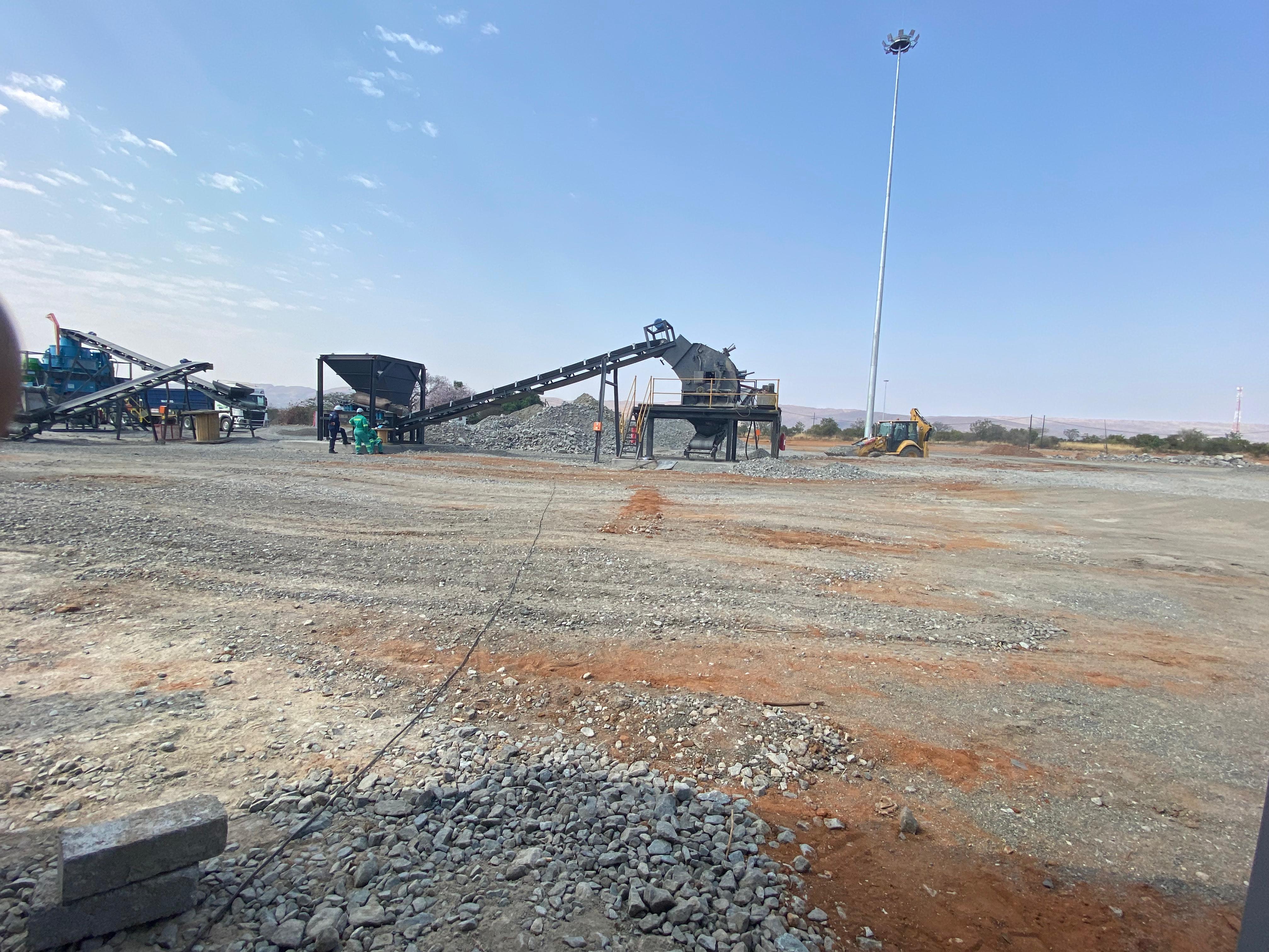
Case Study: Designing for a Crusher and Conveyor System
This case study examines the cabling design for a Horizontal Shaft Impactor (HSI) crusher and three conveyors, providing a practical application of cable failure modes and design principles.
Load Analysis & Current Calculation
The initial step involved calculating the full-load currents (FLC) and applying appropriate safety factors:
- HSI Crusher (180 kW): FLC ≈ 260 A; with a 1.25 safety factor and nameplate power factor, design current ≈ 380 A
- Conveyor 1 (22 kW): FLC ≈ 32 A; design current ≈ 50 A
- Conveyor 2 (18.5 kW): FLC ≈ 27 A; design current ≈ 40 A
- Conveyor 3 (15 kW): FLC ≈ 22 A; design current ≈ 32 A
- Infeed Cable: 300 kVA, current ≈ 502 A
The Direct-On-Line (DOL) starting method for the conveyors resulted in inrush currents of 6–7 times the FLC, making this a critical consideration.
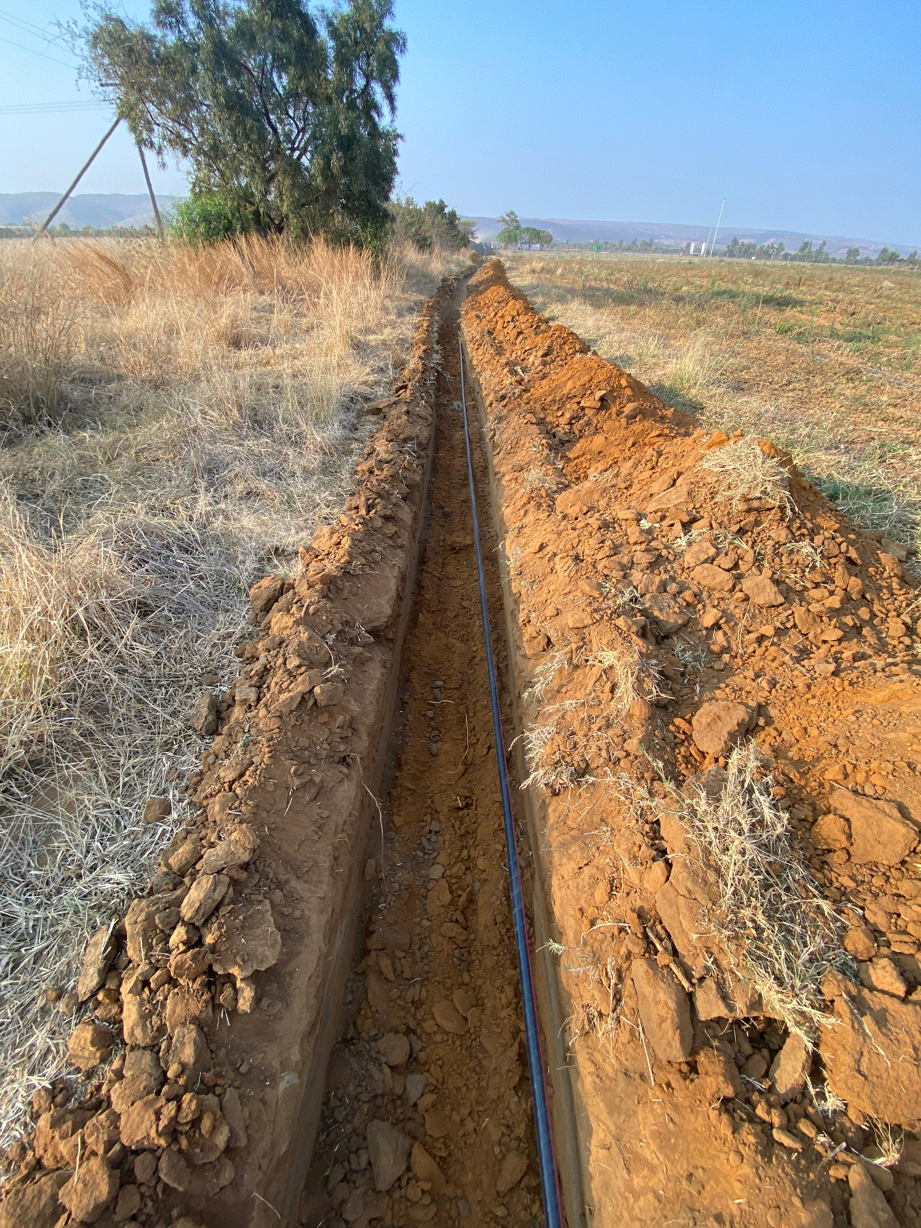
The Dominant Design Factor: Voltage Drop
The 210-meter distance from the substation to the HSI crusher made voltage drop the primary concern. Using the formula V_drop = √3 × I × R × Length, it was evident that for a given cable size (R), the voltage drop over 210 meters would be significant. A cable sized only for ampacity (~600 A) would have resulted in excessive voltage drop. Modeling the voltage drop during soft-start ramp-up was also necessary to ensure proper motor operation and control.
For the conveyors and crusher, shorter cable lengths (60–90 m) reduced voltage drop concerns, but verification was needed to ensure that DOL inrush currents would not cause voltage dips affecting other equipment on the same circuit.
Cable Selection
- Feeder (210 m): 2-Core 300 mm² XLPE/SWA/PVC cable was selected, primarily to minimize resistance and control voltage drop within strict limits (<2.5% at full load), rather than for ampacity alone.
- Conveyor 1 (22 kW, 90 m): 2-Core 16 mm² XLPE/SWA/PVC cable was specified based on ampacity and the need to limit voltage drop during DOL starting.
- Conveyor 2 (18.5 kW, 70 m): 2-Core 16 mm² XLPE/SWA/PVC cable was specified.
- Conveyor 3 (15 kW, 60 m): 2-Core 10 mm² XLPE/SWA/PVC cable was sufficient for the current and inrush requirements.
This project demonstrates that cable design is a negotiation between constraints. For the long run to the crusher, voltage drop was the dominant factor. For the shorter conveyor runs, ampacity and inrush current handling were decisive. Applying theoretical principles ensured a reliable and efficient system that operated correctly under all conditions.
Project Gallery
Conclusion
Now, you're probably wondering: if current dictates the size, how are power lines for entire cities not impossibly thick? We've established that the cross-sectional area of a cable depends on the current it must carry. The key to managing this is to make that current as small as possible. This is where transformers come in—they're the genius behind the entire grid.
At the generator station, voltage is stepped up by massive transformers to incredibly high levels—as high as 765,000 V (765 kV) or more for long-distance transmission. Remember our power equation: P = VI. For a given amount of power (P), increasing voltage (V) drastically decreases current (I). By stepping up the voltage, we reduce the current flowing through those long-distance lines to surprisingly low values—often just a few hundred amperes even for powering entire regions. This allows engineers to use conductors only a few centimeters in diameter, rather than the meters-thick cables that would otherwise be required.
Additionally, this high-voltage, low-current approach is incredibly efficient because it minimizes the dominant loss in transmission lines: I²R losses. The power lost as heat is proportional to the square of the current. Halving the current reduces these losses to a quarter.
Therefore, the entire power grid is a carefully orchestrated dance of voltage:
- Step up to ultra-high voltage for efficient long-distance travel.
- Step down at regional substations for distribution (e.g., to 11kV or 33kV).
- Step down again by a transformer on a pole near your home to the safe voltage we use (230V or 120V).
So, the humble cable's design is ultimately what shaped the architecture of our entire electrical world, forcing the invention of a high-voltage transmission system to make it all feasible.